Graphing Linear Inequalities
Your simple guide to graphing linear inequalities in 3 easy steps

Guide Preview: Graphing Linear Inequalities in 3 Easy Steps
Welcome to this simple and straightforward guide to graphing linear inequalities on the coordinate plane. By the end of this guide, you will be able to:
Graph a linear inequality on the coordinate plane
Identify the solution set of a linear inequality
By working through three examples, you will gain experience and understanding of both of these skills.
However, before going forward, make sure that you are familiar with graphing linear equations in y=mx+b form where m represents the slope and b represents the y-intercept.
Graphing linear inequalities is similar to graphing linear equations (with a few extra steps) and this pre-requisite knowledge is required. If you need a recap of graphing lines in y=mx+b form, we suggest that you review our free Graphing Lines Using Slope step-by-step guide for students.
Once you are able to graph a linear equation in y=mx+b form, you are ready to start graphing linear inequalities in y>mx+ b (or y<, y≥, y≤ form).
But first, let’s quickly review some important math concepts and definitions related to linear relationships and inequalities that will help you along the way.
Equations vs. Inequalities: What is the difference?
Equations
Let’s start by considering the equation x+5=8. Using simple algebra, you can figure out that the solution to this equation is x=3 (see Figure 01).

Figure 01: 3 is the only possible solution to this equation
For this equation, 3 is the only possible solution that would make the equation true and all other values would not work (we can these values non-solutions).
Key Takeaway: Equations can have only one possible solution.
Inequalities
What if we change the equation x+5=8 to the inequality x+5≥8? Using algebra, you can conclude that the solution to the inequality is x≥3.
The solution x≥3 means the value 3 and any value greater than 3 is a possible solution. And there are an infinite amount of values that satisfy this criteria. This infinite set of values that could be solutions to an inequality is called the solution set.
Additionally, if we change the inequality from ≥ to > as follows: x+5>8, you can conclude that the solution to the inequality is x>3.
The solution x>3 means that any value greater than 3 is a possible solution, but not including 3.
You can visualize the solutions to x+5≥8 and x+5>8 on the number line as shown in Figure 02 (the distinction between the solutions of ≥/≤ and >/< inequalities is important to understand before moving forward).
Key Takeaway: Inequalities can have an infinite amount of possible solutions.
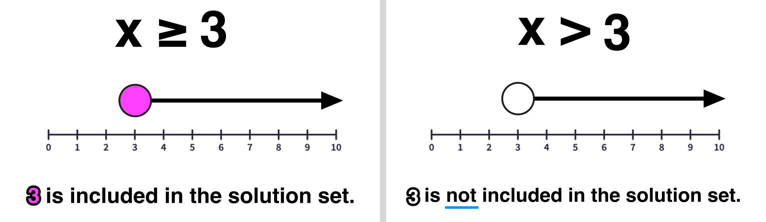
Figure 02: Understand the difference to the solution set for the ≥/≤ and >/< inequality symbols
What does the graph of a linear inequality look like?
Next, we can ask what do linear inequalities and their solution sets look like on the coordinate plane?
Let’s again start with your understanding of linear equations and then building upon it to help you to understand linear inequalities.
For example, consider the linear equations
y=2x+1 and y=2x-1
Both of these linear equations are in y=-mx+b form where m represents the slope and b represents the y-intercept. The first equation has a slope of positive 2 and y-intercept at 1 and the second equation has a slope of negative 2 and y-intercept at 1.
Figure 03 below shows what the graphs of these linear equations looks like:

Figure 03
Next, let’s change both equations to inequalities as follows:
y≥2x+1 and y≤2x-1
These linear inequalities are in y≥mx+b and y≤mx+b form. In fact, they are very similar to their equation counterparts in that the first inequality has a slope of positive 2 and y-intercept at 1 and the second inequality has a slope of negative 2 and y-intercept at 1.
Figure 04 below shows what graphing these linear inequalities looks like:

Figure 04
Notice that the graphs of the equations and the graphs of the inequalities have the same lines, but that the inequality includes shaded region.
Why? When you graph a linear equation, all of the points on the line are solutions to the equation, while all of the points that are not on the line are non-solutions. When you graph a linear inequality, points on the line can be solutions (more on this later) as well as all of the points in the shaded region, which is called the solution set.
At this point, it should also be noted that, just like inequalities on the number line graphs, there is a difference between the solution sets of ≥/≤ and >/< inequalities. Namely, that the solution set of ≥/≤ inequalities includes points on the line, while >/< inequalities do not include points on the line.
On a number line ≥/≤ inequalities have a closed circle and >/< inequalities have an open circle. On the coordinate plane, ≥/≤ linear inequalities have a solid line and >/< linear inequalities have a dotted line.
Are you confused? That’s okay. Let’s take a deeper look at the difference between solid and dotted lines as well as when to shade above or shade below an inequality.
Graphing Linear Inequalities: Lines and Shading
Solid Lines vs. Dotted Lines:
A solid line represents an inclusive boundary. Solid lines are seen in inequalities that use ≤ or ≥, meaning numbers on the line are included in the solution set.
A dotted line represents a non-inclusive boundary. Dotted lines are seen in inequalities that use < or >, meaning numbers on the line are not included in the solution set.
Example: Figure 05 below compares the linear inequalities y>x+1 and y≥x+1. Notice that both inequalities have a shaded region and that y>x+1 has a dotted line, while y≥x+1 has a solid line.

Figure 05
Shading Above vs. Shading Below
The shaded region of a linear inequality includes all of the points that are solutions to the inequality. Any point outside of this shaded region are non-solutions. If the line is solid, then the points on the line are included in the solution set. If the line is dotted, then the points on the line are not included in the solution set.
How do you know when to shade the region above the line or below the line?
When a linear inequality is in the form y> or y≥, shade the area above the graph. All of the points in this region will be solutions to the inequality. Points that sit on the line are included in the solution set only if the line is solid. (Hint: Greater Than ⇾ Shade Above)
When a linear inequality is in the form y< or y≤, shade the area below the graph. All of the points in this region will be solutions to the inequality. Points that sit on the line are included in the solution set only if the line is solid. (Hint: Less Than ⇾ Shade Below)
Figure 06 summarizes exactly when to shade above/below and when a line should be solid/dotted. Once you understand these two important characteristics of linear inequalities, you are ready for your first example problem.
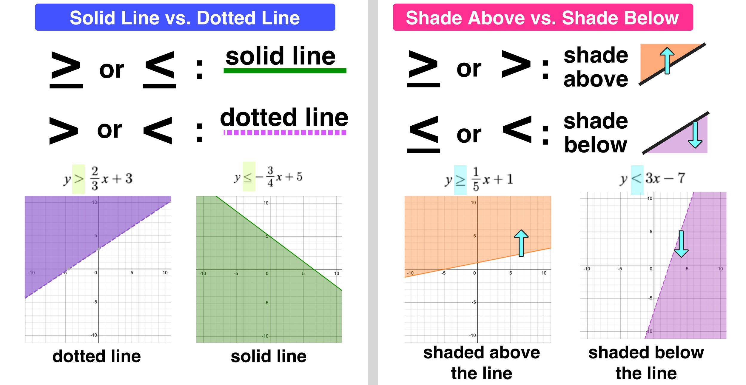
Figure 06
Graphing Linear Inequalities Example #1
Example #1: Graph y≥3x-2 on the coordinate plane.
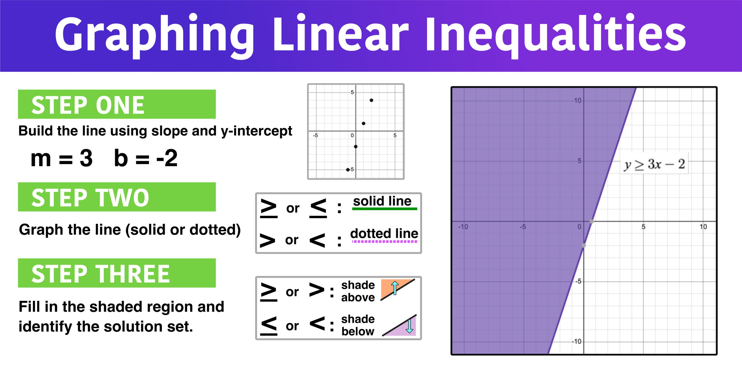
For all of the examples of graphing linear inequalities in this guide, you will be using the following 3-step method:
Step One: “Build the line” by using the slope and y-intercept to plot four or five points on the line.
Step Two: Graph the line (solid if ≥/≤ and dotted if >/<)
Step Three: Shade the region that represents the solution set (shade above if ≥/> and shade below if ≤/<).

Figure 07
Now, let’s apply this 3-step process to Example #1, where you are tasked with graphing the linear inequality y≥3x-2.
Step One: “Build the line” by using the slope and y-intercept to plot four or five points on the line.
This linear equation is of the form y≥mx+b where the slope, m, equals 3 (or 3/1) and the y-intercept is at -2. To build this line, start by plotting a point at the y-intercept (0, -2) and then using the slope (3/1) to plot a few more points on the line. This first step is shown in Figure 08 below.

Figure 08
Step Two: Graph the line (solid if ≥/≤ and dotted if >/<)
Since this linear inequality contains a ≥ symbol, the line that passes through the points will be solid.
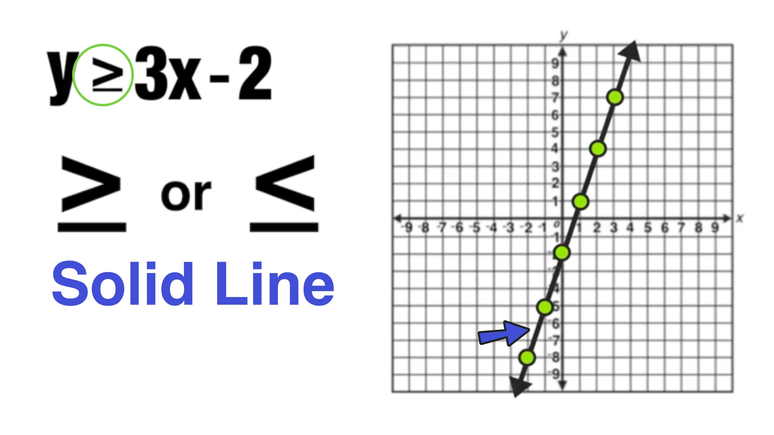
Figure 09
Step Three: Shade the region that represents the solution set (shade above if ≥/> and shade below if ≤/<).
Now that you have your line constructed, the last step is to shade in the solution set region. Since the inequality in this example is ≥, you fill shade above the line as shown in Figure 10 below:

Figure 10A
You have just graphed the linear inequality y≥3x-2.

Figure 10B: The graph of y≥3x-2
Now, let’s take a look at one more example of graphing linear inequalities using our 3-step process.
Graphing Linear Inequalities Example #2
Example #1: Graph y<-1/2x+4 on the coordinate plane.
Step One: “Build the line” by using the slope and y-intercept to plot four or five points on the line.
In this example, the linear inequality is in the form y<mx+b where the slope, m, is -1/2 and the y-intercept is at positive 4 (which means that the line intersects the y-axis at the point (0,4)).
You can start by plotting the y-intercept at (0,4) and then using the slope to build a few more points on the line. Since this line has a negative slope, it should appear to be decreasing from left to right.

Figure 11
Step Two: Graph the line (solid if ≥/≤ and dotted if >/<)
Since this linear inequality contains a < symbol, the line that passes through the points will be dotted.

Figure 12
Step Three: Shade the region that represents the solution set (shade above if ≥/> and shade below if ≤/<).
Now you are ready for shading. Since this linear inequality contains the < symbol, you have to shade in the region below the line as shown in Figure 13 below:
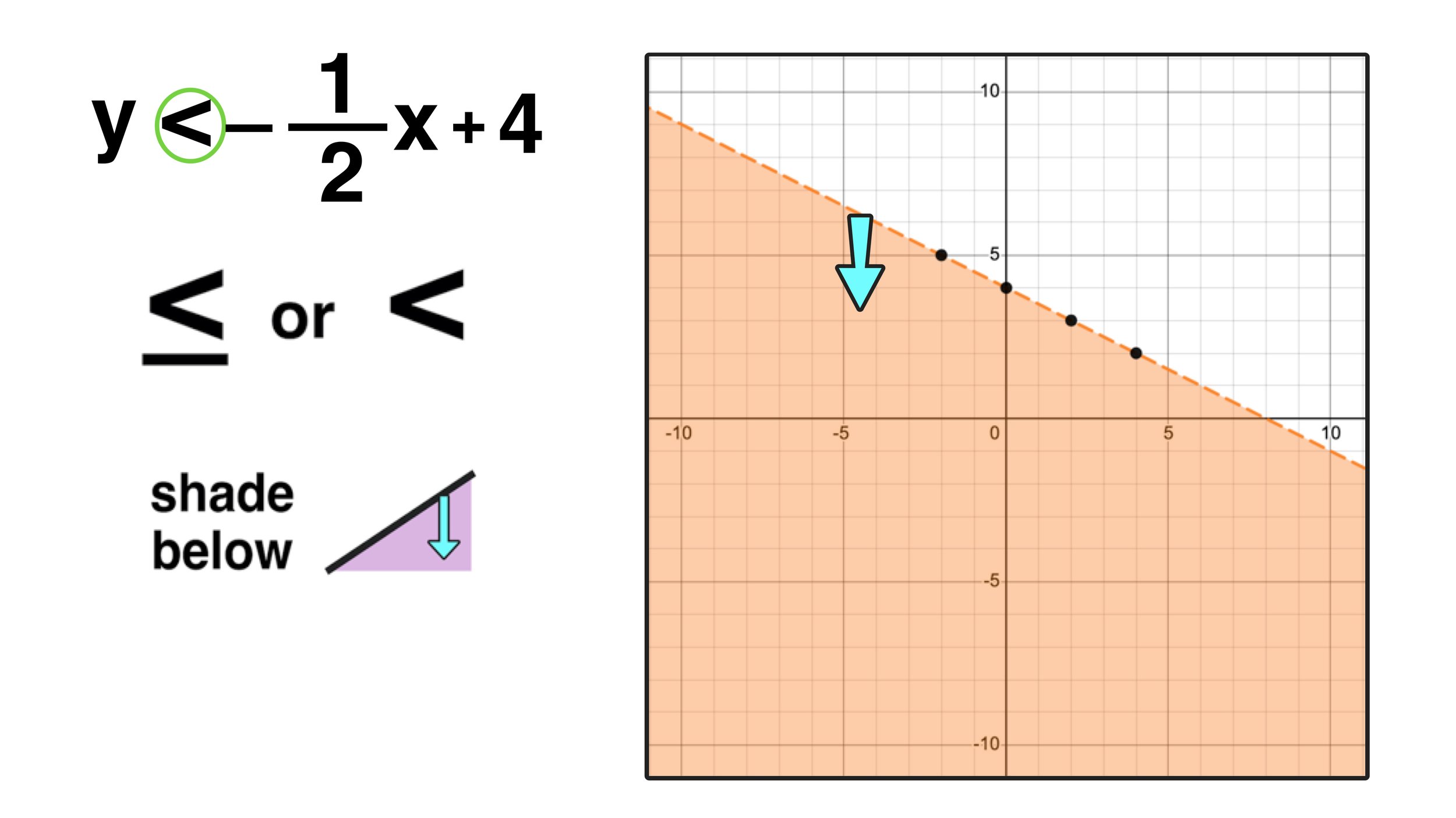
Figure 13A
You’re finished! You have just completely graphed the linear inequality y<-1/2x+4.
Figure 13B: The completed graph of y<-1/2x+4
Need some more practice? Let’s take a look at one more example.
Graphing Linear Inequalities Example #3
Example #1: Graph y>-3/5x-3 on the coordinate plane.
Step One: “Build the line” by using the slope and y-intercept to plot four or five points on the line.
In this example, the linear inequality is in the form y>mx+b where the slope, m, is -3/5 and the y-intercept is at -3.
Go ahead and plot the y-intercept at (0,-3) and then use the slope to construct a few more points.
Step Two: Graph the line (solid if ≥/≤ and dotted if >/<)
Since this linear inequality contains a > symbol, the line that passes through the points will be dotted.

Figure 14: After completing Step One and Step Two.
Step Three: Shade the region that represents the solution set (shade above if ≥/> and shade below if ≤/<).
The final step is to shade the solution set region. Graphing this linear inequality correctly requires you to shade in the region above the line since the inequality symbol is >.
After shading above the line, the result will be that you have completed graphing linear inequality example #3, as shown in Figure 15 below:

Figure 15: The graph of the linear inequality y>-3/5x-3
Conclusion: Graphing Linear Inequalities in Two Variables
Graphing linear inequalities on the coordinate plane is similar to graphing linear equations in the form y=mx+b, but with a few extra steps. The graphs of linear inequalities include a shaded region that represents the linear inequality’s solution set—a region that contains all of the points that satisfy the inequality. Inequalities can also have solid or dotted lines depending on what type of inequality symbol is present. Points on solid lines are included in the solution set, while points are dotted lines are not included in the solution set.
You can graph a linear inequality on the coordinate plane by applying the following 3-step method:
Step One: “Build the line” by using the slope and y-intercept to plot four or five points on the line.
Step Two: Graph the line (solid if ≥/≤ and dotted if >/<)
Step Three: Shade the region that represents the solution set (shade above if ≥/> and shade below if ≤/<).
Below is a visual review of the 3 linear inequalities that you graphed in the guide.

Need more practice with linear inequalities?
More Math Resources You Will Love: