Graphing Systems of Inequalities

Your easy guide to graphing and solving systems of inequalities

In math, once you have learned how to graph and solve a system of linear equations, you are ready to take the next step and learn two new important algebra skills:

Graphing Systems of Inequalities
Solving Systems of Inequalities

This guide will teach you both skills. However, it is important to note that graphing systems of inequalities involves a graphical approach that you may not have explored before.

If you are not confident in your ability to graph and solve a system of linear equations we suggest that review our free Solving Systems of Equations guide.

If you already know how to graph a system of equations, you are ready to follow this step-by-step guide that will teach you everything you need to know about graphing systems of linear inequalities.

Before we dive into solving systems of inequalities, let’s review some definitions and learn the standard notations used when graphing systems of inequalities.

What is the difference between an equation and an inequality?

Definition: An equation is a mathematical statement showing that two expressions are equal using the sign: =

An example of an equation is x=7 where x equals 7 (and only 7).

We can visualize the equation x=7 on the number in Figure 01 below:

Equations have only one possible solution. The equation x=7 means that x must equal 7 and no other value.

Definition: An inequality is a relationship between two values, variables, or expressions making a non-equal comparison

An example of an inequality is x≥7 where x can be equal to 7 or any value larger than 7 (Figure 02).

Inequalities have an infinite number of solutions (this collection of possible solutions is called a solution set). The inequality x≥7 means that x can equal 7 or any value greater than 7. For example:

Solution Examples: 7, 7.5, 57, 2,675, etc.
Non-Solution Examples: 6.999, 3, 0, -413, etc.

The key difference between an equation and an inequality is that an equation has only one solution, while an inequality has a solution set with infinitely many solutions. Keeping this in mind will greatly help you to understand graphing and solving linear inequalities.

Standard Notations used for Graphing Systems of Inequalities

There are a couple of notations that you will need to know before we can start graphing systems of inequalities.

For starters, let’s recap how to graph a single linear inequality of the form y>, y≥, y<, or y≤…

Solid Lines and Dotted Lines:

A solid line represents an inclusive boundary - We see this in inequalities that use ≤ or ≥. This means that numbers on the line are included in the solution set.
A dotted line represents a non-inclusive boundary - We see this in inequalities that use < or >. This means that numbers on the line are not included in the solution set.

For example, Figure 03 below shows the difference between the equation y=x+1 and the inequalities y>x+1 and y≥x+1. Notice that the equation does not have a shaded region while both inequalities do have a shaded region. Also notice that y≥x+1 has a solid line while y>x+1 has a dotted line.

Shaded Regions when Graphing Inequalities:

Next, let’s recap the meaning of the shaded region on the graph of any linear inequality. The shaded region includes all of the points that are solutions to the inequality (there are infinitely many of them). All of the points in the non-shaded region are non-solutions. If the line is solid, then the points on the line are included in the solution set. If the line is dotted, then the points on the line are not included in the solution set.

How do you know when to shade the region above the line or below the line?

When an inequality is in the form y> or y≥, you must shade the region above the graph. All of the points in this region will be solutions to the inequality. Points on the line are only included if the line is solid.
When an inequality is in the form y< or y≤, you must shade the region below the graph. All of the points in this region will be solutions to the inequality. Points on the line are only included if the line is solid.

Figure 04 below recaps both solid and dashed lines and when to shade above a line and when to shade below.

If you need more practice with understanding how to graph a single linear inequality, check out our free guide to graphing linear inequalities on the coordinate plane:

Click here to learn how to graph a single linear inequality

If you can graph a single linear inequality, then you are ready to start graphing systems of inequalities.

Graphing Systems of Inequalities: The Solution Set

When solving systems of linear equations, the solution is a point that satisfies all the equations in the system, but for systems of inequalities, it is an entire region on the coordinate plane. A solution set will have infinitely many points, all of which satisfy every inequality in the system of inequalities.

In Figure 05 below, you can see that the one and only solution to the system of linear equations is the intersection point (5,2). However, for the system of linear inequalities, you can see that all of the points in the overlapping shaded regions can be solutions and there are infinitely many of them. Examples of solutions to the system of inequalities would be the points (0,0), (-2,2 ), and (-4,-1), since they are all in the solution set region, which is labeled with an ‘S'.”

Are you confused? That’s okay for now. Graphing systems of inequalities will become easier for you after working on a few examples. Let’s get started!

Graphing Systems of Inequalities: Example #1

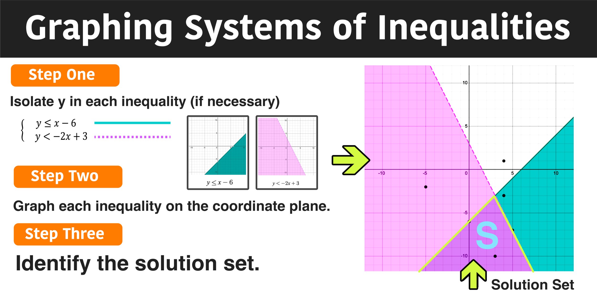
Graph the following system of inequalities:

y ≤ x – 6 and y < –2x + 3

For all of the examples in this guide, you will be graphing the system of inequalities using the following 3-step method:

Step One: Solve both inequalities for y (if necessary). i.e. isolate y as y>, y≥, y<, or y≤
Step Two: Graph both inequalities on the coordinate plane.
Step Three: Determine the solution set.

Now let’s go ahead and apply this 3-step method to example #1:

Step One: Solve both inequalities for y (if necessary). i.e. isolate y as y>, y≥, y<, or y≤

Notice that both of the given inequalities y ≤ x – 6 and y < –2x + 3 already have the y-variable isolated, so there’s nothing that you have to do.

y ≤ x – 6
y < –2x + 3

Step Two: Graph both inequalities on the coordinate plane.

Now you are ready to graph both inequalities. You already know how to graph a single inequality. In this case, you are just graphing them both on the same graph so that you can see where the shaded regions overlap.

Figure 06 below shows what the graphs of y ≤ x – 6 and y < –2x + 3 would look on separate graphs and what graphing the system of inequalities would look like on the same coordinate with the overlapping region marked with an S, which represents the solution set.

Step Three: Determine the solution set.

Now that you have graphed both inequalities on the coordinate plane, you are ready to determine the solution set. Any point contained within the overlapping region will be a solution and satisfy both inequalities.

Observe Figure 07 below to see the difference between the region of the graph that represents the solution set and the region remaining region that contains all of the non-solutions. Note that points on a solid line within the solution set are included in the solution set, while points on a dotted line are not.

With this key concept to graphing systems of inequalities in mind, you can now determine that the solution set is the overlapping region that you will mark with the letter S.

To recap, Figure 08 below shows what the completed graph should look like:

As far as solving systems of linear inequalities goes, your graph has done that by demonstrating the solution set—the region that contains all of the points that will satisfy both inequalities.

If you wanted to determine if individual points are in the solution set, you would simply use your graph to see whether or not they are contained within the solution set. For example:

(4,1) is a non-solution because it is not in the solution set ✗
(3, -10) is a solution because it is in the solution set ✓
(-5, -2) is a non-solution because it is not in the solution set ✗
(0,-6) is a solution because it is in the solution set (it is on the solid line portion of the solution set) ✓
(5, -7) is a non-solution because it is not in the solution set (it is on the dotted line portion of the solution set) ✗
(4, -3) is a non-solution because it is not in the solution set ✗

Need some more practice? Let’s take a look at another example.

Graphing Systems of Inequalities: Example #2

Graph the following system of inequalities:

y ≤ 3x - 5 and 2y - 5 > x -3

Just like the last example, you will be following the 3-step method as follows:

Step One: Solve both inequalities for y (if necessary). i.e. isolate y as y>, y≥, y<, or y≤

This step involves rearranging each inequality such that y is the subject of the inequality.

In this example, the first inequality is already in the desired form. Rearrange the second inequality as follows:

2y - 5 > x -3
+5 to both sides → 2y - 5 + 5 > x - 3 + 5 = 2y > x + 2
2y > x + 2
/2 on both sides → 2y/2 > x/2 + 2/2 = y > (½)x + 1
= y > (½)x + 1

You have now isolated y in the second inequality and are ready to start solving systems of inequalities: y ≤ 3x - 5 and y > (½)x + 1.

Step Two: Graph both inequalities on the coordinate plane.

Now you are ready to graph y ≤ 3x - 5 and y > (½)x + 1 on the same graph. Remember that:

y ≤ 3x - 5 will have a solid line and the shaded region will be below the line.
y > (½)x + 1 will have a dotted line and the shaded region will be above the line.

Just like the first example, we can visualize graphing each linear inequality on a separate graph and the together, overlapping, on the same graph as is shown in Figure 09 below.

Step Three: Identify the solution set.

Finally, the solution set for the given system of linear inequalities lies in the region where the solution sets of each individual inequality overlap. This overlapping region is shown below in Figure 10.

Graphing the system of inequalities is completed and you have identified the solution set.

Again, if you could check individual points that satisfy both inequalities as follows:

(4,7) is a solution because it is in the solution set (it is on the solid line portion of the solution set) ✓
(8, 8) is a solution because it is in the solution set ✓
(4, 4) is a non-solution because it is not in the solution set (it is on the dotted line portion of the solution set) ✗
(4,5) is a solution because it is in the solution set ✓
(0,0) is a non-solution because it is not in the solution set ✗
(-3, 6) is a non-solution because it is not in the solution set ✗

Are you feeling more comfortable with the three-step process? Luckily, this process works for graphing systems of inequalities in two variables and solving systems of inequalities in two variables, so, once you get it down, you can solve any example. Let’s put your skills to the test with one final example.

Graphing Systems of Inequalities: Example #3

Graph the following system of inequalities:

6x - 2y ≥ -10 and 8 + y < 10

Step One: Solve both inequalities for y (if necessary). i.e. isolate y as y>, y≥, y<, or y≤

In this example, you will have to use algebra to rearrange both inequalities since neither is in the desired form.

Starting with the first inequality:

6x - 2y ≥ -10
-6x to both sides → -6x + 6x - 2y ≥ -10 - 6x = -2y ≥ -6x - 10
-2y ≥ -6x - 10
/-2 on both sides → -2y/-2 ≥ -6x/-2 - 10/-2 → y ≤ 3x + 5 (Did you notice that the inequality sign changes from ≥ to ≤ 😮)
***Note that whenever you divide and inequality by a negative number (-2 in this example), the inequality sign reverses direction.
= y ≤ 3x + 5

You have now isolated y in the first inequality and can conclude that y ≤ 3x + 5

And now for the second equation:

8 + y < 10
-8 from both sides → -8 +8 + y < 10 - 8 = y<2
y<2

You have now isolated y in the second inequality and can conclude that y < 2

Step Two: Graph both inequalities on the coordinate plane.

Now you are ready to graph y ≤ 3x + 5 and y < 2 on the same graph. Remember that:

y ≤ 3x + 5 will have a solid line and the shaded region will be below the line.
y < 2 will have a dotted line and the shaded region will also be below the line.

Step Three: Identify the solution set.

Now you can identify the solution set for the graph of the system of inequalities. This region where the solution set for both inequalities is shown in the graph below in Figure 12:

The final graphing systems of inequalities example is now complete.

Let’s take a look at some points and determine whether or not they are in the solution set.:

(-2,-1) is a solution because it is in the solution set (it is on the solid line portion of the solution set) ✓
(9, -5) is a solution because it is in the solution set ✓
(5, 2) is a non-solution because it is not in the solution set (it is on the dotted line portion of the solution set) ✗
(0,0) is a solution because it is in the solution set ✓
(10,10) is a non-solution because it is not in the solution set ✗
(-2, 0) is a non-solution because it is not in the solution set ✗

Conclusion

Graphing systems of inequalities and solving systems of inequalities can be done easily by adhering to the following 3-step meth:

Step One: Solve both inequalities for y (if necessary). i.e. isolate y as y>, y≥, y<, or y≤

Step Two: Graph both inequalities on the coordinate plane.

Step Three: Identify the solution set.

Even though this guide showed examples involving systems of inequalities with two inequalities, you can follow the same steps to solve a system with any number of inequalities. If you are familiar with graphs of nonlinear functions, you can transfer the knowledge gained in this guide to solve systems of inequalities that include higher-order inequalities too.